Conformal Transformations

Tilings generated with hypertiling can be transformed beyond the usual Poincaré disk representation using conformal mappings. A conformal map is a function that preserves angles locally, meaning it maintains the angles and shapes of infinitesimally small figures. As a result, the overall pattern’s outline remains unchanged before and after the mapping.

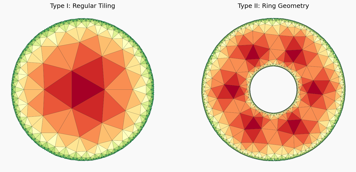
By applying specific conformal mappings, we generate what is known as a type-II hyperbolic lattice. This structure is mathematically equivalent to a constant-time slice of a three-dimensional BTZ black hole. In this demo notebook, we illustrate how these mappings work and explore the resulting geometric transformations.

Further reading:

• Chen, Jingming, et al. “AdS/CFT correspondence in hyperbolic lattices.” arXiv:2305.04862 (2023). URL: https://arxiv.org/abs/2305.04862

• Dey, Santanu, et al. “Simulating holographic conformal field theories on hyperbolic lattices.” Physical Review Letters 133.6 (2024): 061603. URL: https://doi.org/10.1103/PhysRevLett.133.061603

• Ouyang, Peichang, et al. “Automatic generation of hyperbolic drawings.” Applied Mathematics and Computation 347 (2019): 653-663. URL: https://doi.org/10.1016/j.amc.2018.09.052

from hypertiling import HyperbolicTiling
import matplotlib as mpl
import matplotlib.pyplot as plt
import numpy as np


def generate_color_palette(colormap_name, num_samples):
    cmap = plt.get_cmap(colormap_name)  # Get the colormap
    colors = [cmap(i) for i in np.linspace(0, 1, num_samples)]  # Generate color samples
    hex_colors = [mpl.colors.to_hex(color) for color in colors]  # Convert to hex
    return hex_colors

Let us define the conformal mappings we need

disc2stripe = np.vectorize(lambda z: 2 / np.pi * np.log((1 + z) / (1 - z)))
stripe2ring = np.vectorize(lambda z, k, delta: np.exp(2 * np.pi * 1j * (z + 1j) / (k * delta)))

Reusable function for plotting

def plot_conformal_tiling(ax, tiling, k, delta=1.845, squash=True, wrap=True):
    """
    Draws the tiling on the given axis (ax) with parameter k.
    Default parameters correspond to (3,7) tiling
    """

    fund_region = [-delta/2, delta/2]

    if wrap and not squash:
        squash = False

    for i in range(k):
        for idx, pgon in enumerate(tiling):

            if squash:
                pgonn = disc2stripe(pgon)

                # Exclude polygons outside the fundamental region
                if np.real(pgonn[0]) < fund_region[0] or np.real(pgonn[0]) > fund_region[1]:
                    continue

                # Replicate along the stripe
                pgonn += i * delta

            else:
                pgonn = pgon

            # Color by reflection level
            poly_layer = tiling.get_reflection_level(idx)
            facecolor = generate_color_palette('RdYlGn', nlayers + 1)[poly_layer]

            # Apply second conformal transformation
            if wrap:
                pgonn = stripe2ring(pgonn, k, delta)

            # Draw polygon
            patch = mpl.patches.Polygon(np.array([(np.real(e), np.imag(e)) for e in pgonn[1:]]),
                                        facecolor=facecolor, edgecolor="black", linewidth=0.15)
            ax.add_patch(patch)

BTZ Black Hole

# Create a single tiling for both types
# the way the first transformations are formulated, make sure the lattice is
# rotationally aligned to the x-axis; which can be done setting mangle=0
nlayers = 12
tiling = HyperbolicTiling(3, 7, nlayers, kernel="GR", mangle=0)

# Create figure and axes for side-by-side subplots
fig, (ax1, ax2) = plt.subplots(1, 2, figsize=(14, 7), dpi=130)

delta = 1.845 # found by hand, could be automatically computed though

# Type I: Regular Tiling
plot_conformal_tiling(ax1, tiling, 1, squash=False, wrap=False)

# Type II: Ring Geometry
plot_conformal_tiling(ax2, tiling, 6, delta=delta, squash=True, wrap=True)


# Common figure adjustments
for ax in [ax1, ax2]:
    ax.set_xlim(-1.1, 1.1)
    ax.set_ylim(-1.1, 1.1)
    ax.set_box_aspect(1)
    ax.set_axis_off()
fig.patch.set_facecolor('#F9F9F9')


ax1.set_title("Type I: Regular Tiling", fontsize=14)
ax2.set_title("Type II: Ring Geometry", fontsize=14)
plt.show()

Replications

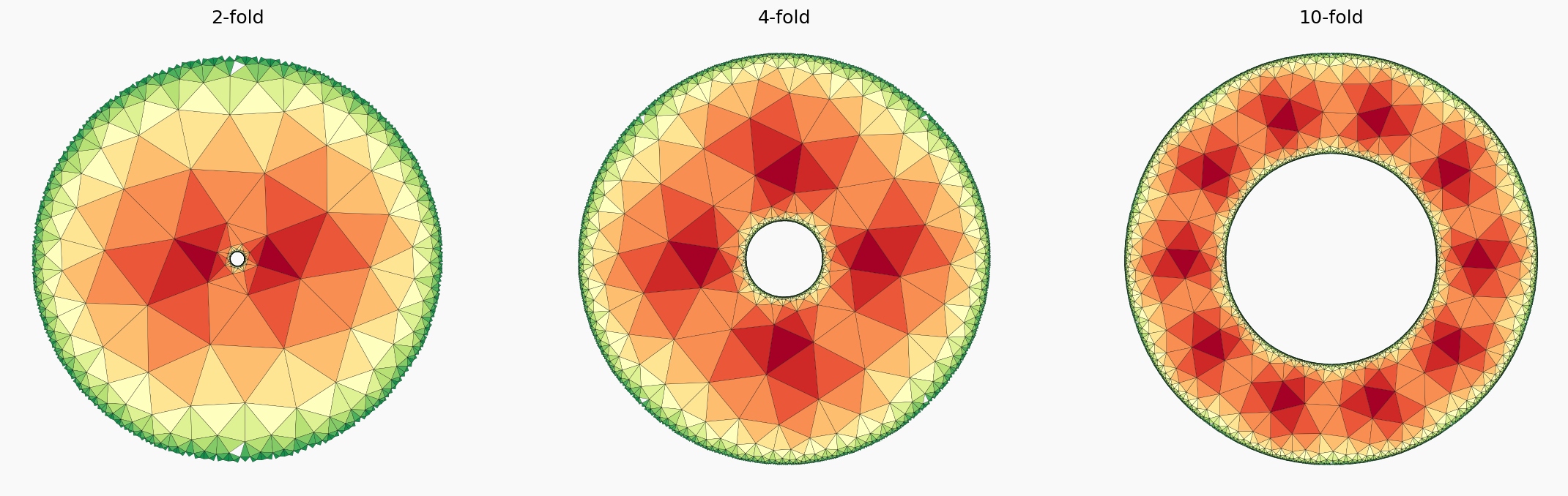
Changing the k parameter will produce type-II tilings which are less or more curved towards the singularities

delta = 1.845

nlayers = 12
tiling = HyperbolicTiling(3, 7, nlayers, kernel="GR", mangle=0)

# Create figure and axes for three subplots
fig, (ax1, ax2, ax3) = plt.subplots(1, 3, figsize=(21, 7), dpi=130)

# plot the tilings
plot_conformal_tiling(ax1, tiling, k=2, delta=delta)
plot_conformal_tiling(ax2, tiling, k=4, delta=delta)
plot_conformal_tiling(ax3, tiling, k=10, delta=delta)

# Common figure adjustments for all subplots
for ax in [ax1, ax2, ax3]:
    ax.set_xlim(-1.1, 1.1)
    ax.set_ylim(-1.1, 1.1)
    ax.set_box_aspect(1)
    ax.set_axis_off()
fig.patch.set_facecolor('#F9F9F9')

ax1.set_title("2-fold", fontsize=14)
ax2.set_title("4-fold", fontsize=14)
ax3.set_title("10-fold", fontsize=14)
plt.show()

Step by Step

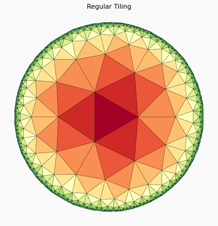
Now we apply the transformation step by step. We start with the regular (3,7) tiling

nlayers = 12
tiling = HyperbolicTiling(3, 7, nlayers, kernel="GR", mangle=0)

# Create figure and axes, adjust background
fig, ax = plt.subplots(figsize=(7,7), dpi=130)
ax.set_xlim(-1.1, 1.1)
ax.set_ylim(-1.1, 1.1)
ax.set_box_aspect(1)
ax.set_axis_off()
fig.patch.set_facecolor('#F9F9F9')


# Loop through polygons
for idx, pgon in enumerate(tiling):

    # color by layer
    poly_layer = tiling.get_reflection_level(idx)
    facecolor = generate_color_palette('RdYlGn', nlayers+1)[poly_layer]

    # draw polygon
    patch = mpl.patches.Polygon(np.array([(np.real(e), np.imag(e)) for e in pgon[1:]]),
                                facecolor=facecolor, edgecolor="black", linewidth=0.3)
    ax.add_patch(patch)

# Show plot
plt.title("Regular Tiling")
plt.show()

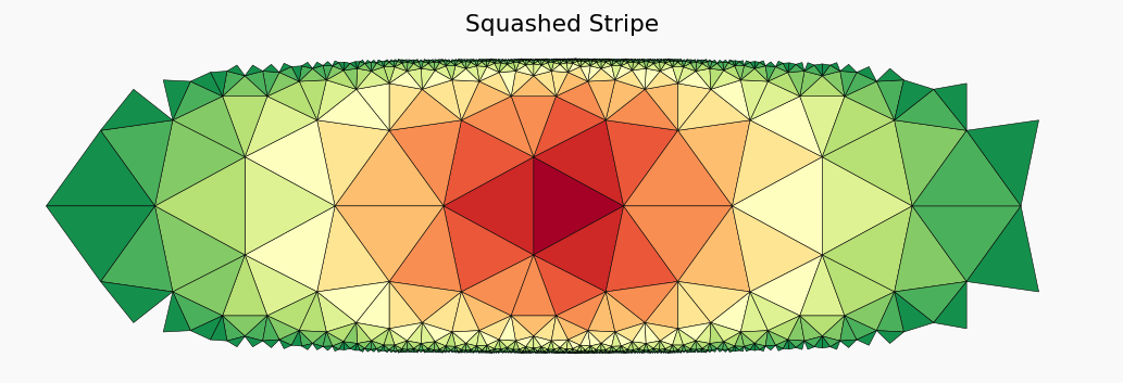
We apply the conformal transformation $ C_1 $ from Poincaré disk to stripe coordinates:

$ C_1 : z \mapsto `:nbsphinx-math:zeta = :nbsphinx-math:frac{2}{pi}` \ln `:nbsphinx-math:left`( \frac{1 + z}{1 - z} \right) $

where domain and range are $ C_1 : \mathbb{D} \to `:nbsphinx-math:mathbb{B}` = { \zeta `:nbsphinx-math:in :nbsphinx-math:mathbb{C}` \mid `\|:nbsphinx-math:Im`(\zeta)| < 1 } $

delta = 1.845 # length of the periodic block
k = 1

nlayers = 12
tiling = HyperbolicTiling(3, 7, nlayers, kernel="GR", mangle=0)

# Create figure and axes, adjust background
fig, ax = plt.subplots(figsize=(10,3), dpi=130)
ax.set_xlim(-3.5, 3.5)
ax.set_ylim(-1.1, 1.1)
ax.set_axis_off()
fig.patch.set_facecolor('#F9F9F9')

# Number of replications
for i in range(k):

    # Loop through polygons
    for idx, pgon in enumerate(tiling):

        # apply 1st conformal mapping
        pgon_stripe = disc2stripe(pgon)

        # color by layer
        poly_layer = tiling.get_reflection_level(idx)
        facecolor = generate_color_palette('RdYlGn', nlayers+1)[poly_layer]

        # draw polygon
        patch = mpl.patches.Polygon(np.array([(np.real(e), np.imag(e)) for e in pgon_stripe[1:]]),
                                    facecolor=facecolor, edgecolor="black", linewidth=0.3)
        ax.add_patch(patch)

# Show plot
plt.title("Squashed Stripe")
plt.show()

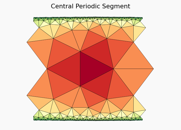
We identify a repeating pattern and cut out one periodic element

delta = 1.845 # length of the periodic block
k = 1

nlayers = 12
tiling = HyperbolicTiling(3, 7, nlayers, kernel="GR", mangle=0)

# Create figure and axes, adjust background
fig, ax = plt.subplots(figsize=(6,4), dpi=130)
ax.set_xlim(-1.5, 1.5)
ax.set_ylim(-1.1, 1.1)
ax.set_axis_off()
fig.patch.set_facecolor('#F9F9F9')

# Number of replications
for i in range(k):

    # Loop through polygons
    for idx, pgon in enumerate(tiling):

        # apply 1st conformal mapping
        pgon_stripe = disc2stripe(pgon)

        # vertical cut: withdraw polygons with centers ouside "fundamental" region
        if np.real(pgon_stripe[0]) < -0.98 or np.real(pgon_stripe[0]) > 0.9:
            continue

        # color by layer
        poly_layer = tiling.get_reflection_level(idx)
        facecolor = generate_color_palette('RdYlGn', nlayers+1)[poly_layer]

        # draw polygon
        patch = mpl.patches.Polygon(np.array([(np.real(e), np.imag(e)) for e in pgon_stripe[1:]]),
                                    facecolor=facecolor, edgecolor="black", linewidth=0.3)
        ax.add_patch(patch)

# Show plot
plt.title("Central Periodic Segment")
plt.show()

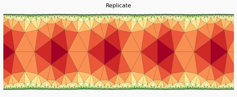
This segment is replicated \(k\) times (in this case \(k=6\))

delta = 1.845 # length of the periodic block
k = 6

nlayers = 12
tiling = HyperbolicTiling(3, 7, nlayers, kernel="GR", mangle=0)

# Create figure and axes, adjust background
fig, ax = plt.subplots(figsize=(9,3.3), dpi=130)
ax.set_xlim(0, 8)
ax.set_ylim(-1.1, 1.1)
ax.set_axis_off()
fig.patch.set_facecolor('#F9F9F9')

# Number of replications
for i in range(k):

    # Loop through polygons
    for idx, pgon in enumerate(tiling):

        # apply 1st conformal mapping
        pgon_stripe = disc2stripe(pgon)

        # vertical cut: withdraw polygons with centers ouside "fundamental" region
        if np.real(pgon_stripe[0]) < -0.98 or np.real(pgon_stripe[0]) > 0.9:
            continue

        # replicate
        pgon_stripe += i * delta

        # color by layer
        poly_layer = tiling.get_reflection_level(idx)
        facecolor = generate_color_palette('RdYlGn', nlayers+1)[poly_layer]

        # draw polygon
        patch = mpl.patches.Polygon(np.array([(np.real(e), np.imag(e)) for e in pgon_stripe[1:]]),
                                    facecolor=facecolor, edgecolor="black", linewidth=0.15)
        ax.add_patch(patch)

plt.title("Replicate")
plt.show()

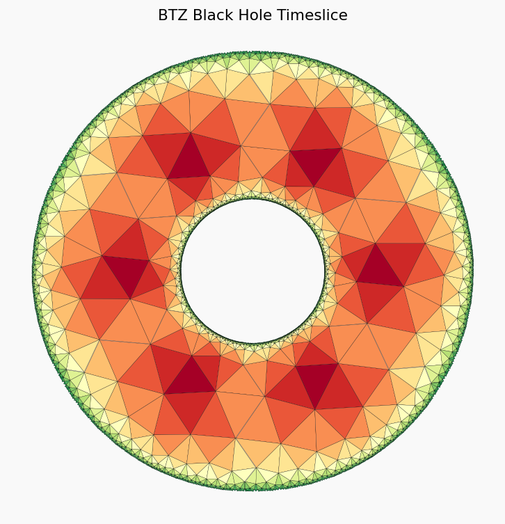
Now we wrap the stripe in order to arrive at a ring geometry using the second conformal transformation

$ C_2 : \zeta `:nbsphinx-math:mapsto :nbsphinx-math:hat{z}` = e^{2:nbsphinx-math:pi `i (:nbsphinx-math:zeta`+i) / (k*:nbsphinx-math:Delta)} $

where domain and range are $ C_1 : \mathbb{B} \to `:nbsphinx-math:mathbb{A}` = { \hat{z} \in `:nbsphinx-math:mathbb{C}` \quad `:nbsphinx-math:hat{r}`_0 < |:nbsphinx-math:hat{z}| < 1 } $

delta = 1.85
k = 6

nlayers = 12
tiling = HyperbolicTiling(3, 7, nlayers, kernel="GR", mangle=0)

# Create figure and axes, adjust background
fig, ax = plt.subplots(figsize=(7,7), dpi=130)
ax.set_xlim(-1.1, 1.1)
ax.set_ylim(-1.1, 1.1)
ax.set_box_aspect(1)
ax.set_axis_off()
fig.patch.set_facecolor('#F9F9F9')

# Number of replications
for i in range(k):

    # Loop through polygons
    for idx, pgon in enumerate(tiling):

        # apply 1st conformal mapping
        pgon_stripe = disc2stripe(pgon)

        # vertical cut: withdraw polygons with centers ouside "fundamental" region
        if np.real(pgon_stripe[0]) < -0.98 or np.real(pgon_stripe[0]) > 0.9:
            continue

        # replicate
        pgon_stripe += i * delta

        # color by layer
        poly_layer = tiling.get_reflection_level(idx)
        facecolor = generate_color_palette('RdYlGn', nlayers+1)[poly_layer]

        # apply 2nd conformal mapping
        pgon_ring = stripe2ring(pgon_stripe[1:], k, delta)

        # draw polygon
        patch = mpl.patches.Polygon(np.array([(np.real(e), np.imag(e)) for e in pgon_ring]),
                                    facecolor=facecolor, edgecolor="black", linewidth=0.15)
        ax.add_patch(patch)

plt.title("BTZ Black Hole Timeslice")
plt.show()

Other Tilings

The transformations can also be applied to other than the (3,7) triangular tiling. The parameter \(\Delta\) needs to be adjusted

from hypertiling.graphics.svg import make_svg, draw_svg

def return_conformal_tiling(tiling, k, delta):
    """
    Draws the tiling on the given axis (ax) with parameter k.
    Default parameters correspond to (3,7) tiling
    """

    fund_region = [-delta/2, delta/2]

    new_tiling = []

    for i in range(k):
        for idx, pgon in enumerate(tiling):

            pgon = disc2stripe(pgon)

            # Exclude polygons outside the fundamental region
            if np.real(pgon[0]) < fund_region[0] or np.real(pgon[0]) > fund_region[1]:
                continue

            # Replicate along the stripe
            pgon += i * delta


            # Apply second conformal transformation
            pgon = stripe2ring(pgon, k, delta)

            new_tiling.append(pgon)


    return new_tiling

Let us create an 8-fold ring geometry of a (4,6) tiling

tiling = HyperbolicTiling(4, 6, 7, kernel="GR", mangle=0)
tiling = return_conformal_tiling(tiling, 8, delta=1.46)
draw_svg(make_svg(tiling, unitcircle=True))

Let us create an 5-fold ring geometry of a (7,4) tiling

tiling = HyperbolicTiling(7, 4, 5, kernel="GR", mangle=0)
tiling = return_conformal_tiling(tiling, 5, delta=3.09)
draw_svg(make_svg(tiling, unitcircle=True))