Refinements

In this notebook, we demonstrate how so-called refinements of hyperbolic tilings can be constructed with hypertiling. Currently, this feature is only supported for triangular tilings and works only in combination with the static rotational kernels (SR and SRI).

import numpy as np
import matplotlib.cm as cmap
import matplotlib.pyplot as plt

from hypertiling import HyperbolicTiling
from hypertiling.graphics.plot import quick_plot, convert_edges_to_arcs
from hypertiling.geodesics import geodesic_arc

This is an example how hyperbolic lattice refinements can be created

# construct tiling using the static rotational (SRS) kernel
TR = HyperbolicTiling(3,7,4, kernel="SRS") # will be refined
TO = HyperbolicTiling(3,7,4, kernel="SRS") # for reference

# add one layer of refinements
TR.refine_lattice(1)

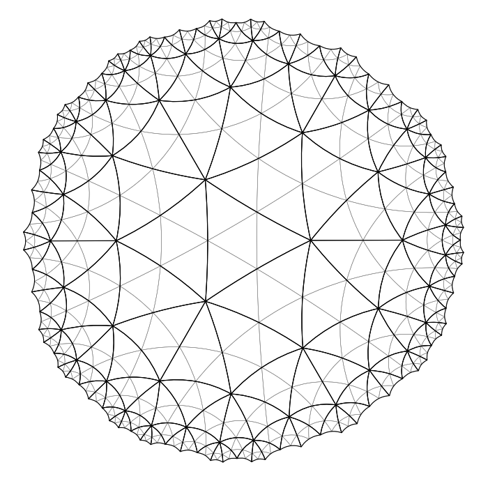
We plot the original cells as thick black lines

# prepare figure
fig, ax = plt.subplots(figsize=(8,7), dpi=100)

# refined lattice
# convert cell edges to matplotlib arcs
edges, types = convert_edges_to_arcs(TR, lw=0.4)
for edge in edges:
    ax.add_artist(edge)
    edge.set_color('grey')

# original lattice
# convert cell edges to matplotlib arcs
edges, types = convert_edges_to_arcs(TO, lw=0.8)
for edge in edges:
    ax.add_artist(edge)
    edge.set_color('black')

plt.xlim(-1,1); plt.ylim(-1,1)
plt.axis("off"); plt.gca().set_aspect('equal')
plt.tight_layout(); plt.show()

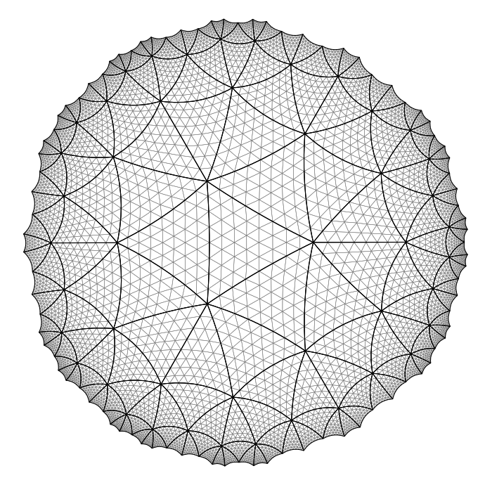
Now let us do some more refinement steps

# construct tiling using the SRS kernel
TR = HyperbolicTiling(3,7,4, kernel="SRS") # will be refined
TO = HyperbolicTiling(3,7,4, kernel="SRS") # for reference

# add one layer of refinements
TR.refine_lattice(3)

# prepare figure
fig, ax = plt.subplots(figsize=(8,7), dpi=100)

# refined lattice
# convert cell edges to matplotlib arcs
edges, types = convert_edges_to_arcs(TR, lw=0.4)
for edge in edges:
    ax.add_artist(edge)
    edge.set_color('grey')

# original lattice
# convert cell edges to matplotlib arcs
edges, types = convert_edges_to_arcs(TO, lw=0.8)
for edge in edges:
    ax.add_artist(edge)
    edge.set_color('black')

plt.xlim(-1,1); plt.ylim(-1,1)
plt.axis("off"); plt.gca().set_aspect('equal')
plt.tight_layout(); plt.show()

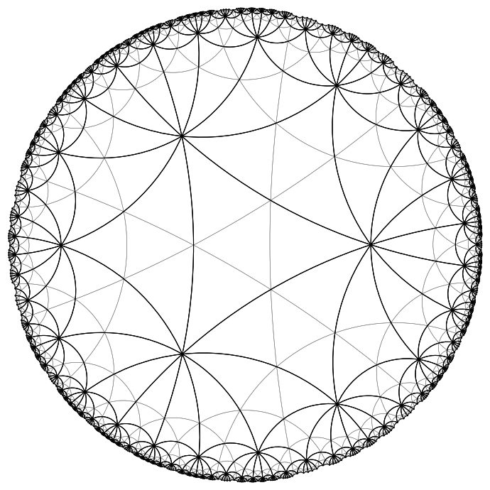
refinements work for any triangular tiling, therefore let us try a different \(q\)

# construct tiling using the SRS kernel
TR = HyperbolicTiling(3,10,4, kernel="SRS") # will be refined
TO = HyperbolicTiling(3,10,4, kernel="SRS") # for reference

# add one layer of refinements
TR.refine_lattice(1)

# prepare figure
fig, ax = plt.subplots(figsize=(8,7), dpi=100)

# refined lattice
# convert cell edges to matplotlib arcs
edges, types = convert_edges_to_arcs(TR, lw=0.4)
for edge in edges:
    ax.add_artist(edge)
    edge.set_color('grey')

# original lattice
# convert cell edges to matplotlib arcs
edges, types = convert_edges_to_arcs(TO, lw=0.8)
for edge in edges:
    ax.add_artist(edge)
    edge.set_color('black')

plt.xlim(-1,1); plt.ylim(-1,1)
plt.axis("off"); plt.gca().set_aspect('equal')
plt.tight_layout(); plt.show()

And even larger \(q\); this time we use a different plot function, since plotting those geodesic arcs is rather slow

# construct tiling using the SRS kernel
TR = HyperbolicTiling(3,12,4, kernel="SRS")

# add one layer of refinements
TR.refine_lattice(3)

# use fast plot function, as the number of cells is quite huge
quick_plot(TR, lw=0.1)

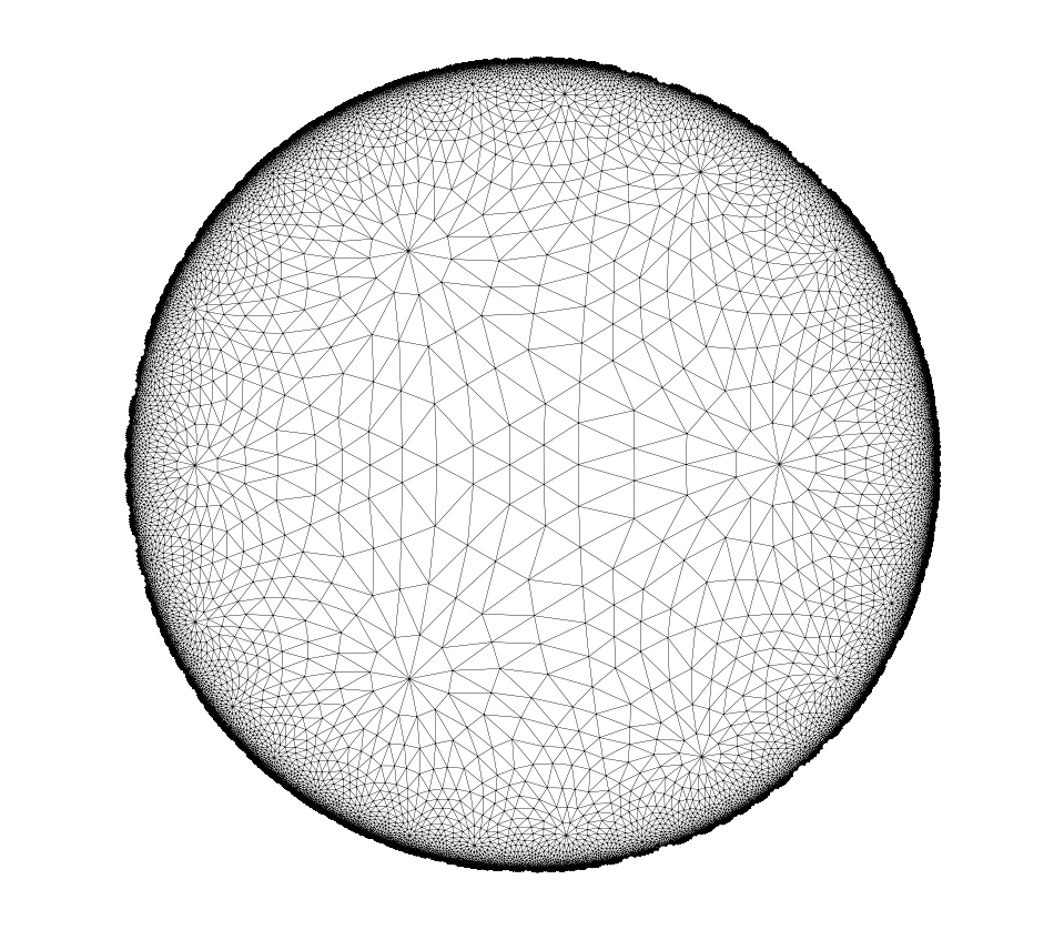
Hint: See also the notebook “advanced-visualization”, where the vector graphics capabilities of hypertiling are demonstrated.