Dynamic Lattice Manipulation

new experimental feature of the SRG kernel

from hypertiling import HyperbolicTiling
from hypertiling.graphics.svg import *
from hypertiling.graphics.plot import plot_geodesic
import matplotlib.pyplot as plt

def myplot(tiling):
    ax = plot_geodesic(T, ec="0.6", lw=0.7, zorder=3)
    for idx, poly in T.polygons.items():
        if idx in T.exposed:
            col = "#ad153d"
        else:
            col = "k"
        z = poly.centerP()
        t = ax.text(np.real(z), np.imag(z), str(idx), c=col, ha="center", va="center", fontsize=17*(1-0.7*np.abs(z)), zorder=1)
        t.set_bbox(dict(facecolor='w', edgecolor="none", alpha=0.5))

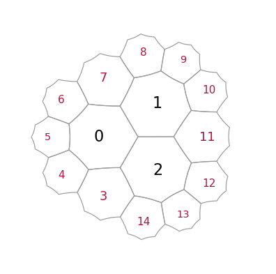
General usage

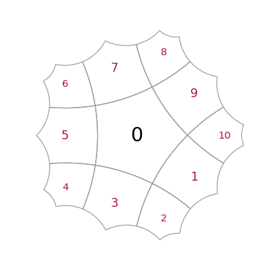
Construct and draw a small lattice to start with. Cells with red labels are called “exposed”, they represent the outmost layer and their neigbours are incomplete as they only know about their parents, but not about siblings

T = HyperbolicTiling(7, 3, 2, kernel="SRG", center="vertex")

myplot(T)

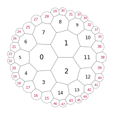
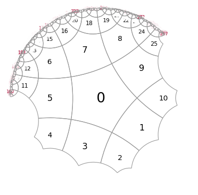
Upon execution of “add_layer”, the vacant spaced around all exposed cells is filled with new polygons

T.add_layer()

myplot(T)

We can also remove cells, using a list of corresponding indices

T.remove_cells([7,8,9,10,11,12,13,14])
T.remove_cells([1])
T.remove_cells(range(27,36))
T.remove_cells(range(37,42))

myplot(T)

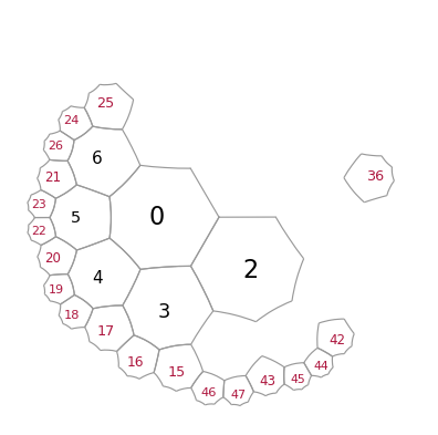
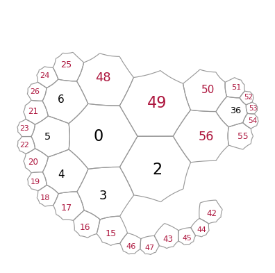
Let us again add a layer to reconnect the pieces

T.add_layer([0,36])

myplot(T)

Filters

The add_layer function allows to use filters, which can specify the domain in which we want to construct new cells

# this filter allows construct cells only in a certain range of complex angles
def my_angular_filter(z):
    return True if (45 < np.angle(z, deg=True) < 180) else False

T = HyperbolicTiling(5,4, 2, kernel="SRG")

myplot(T)

And this is how it works

T.add_layer(filter = my_angular_filter)
T.add_layer(filter = my_angular_filter)
T.add_layer(filter = my_angular_filter)

myplot(T)