As another application of the MARQOV framework, we simulate the \(O(3)\) model on a three-dimensional random geometric graph (RGG, compare Part I), modeling a finite, fixed interaction radius in a disordered medium. The radius is chosen such that on average the nodes have six neighbors, representing moderate to strong disorder.1 Due to the fact that the RGG represents effectively uncorrelated randomness, we can apply Harris’ inequality, according to which disorder should be irrelevant if \(d\nu >2\). Since for the three-dimensional Heisenberg universality class, \(\nu\approx 0.71\)2, the criterion predicts that one should find a clean transition in this case, similar to dilute Heisenberg systems, which already have been investigated3.
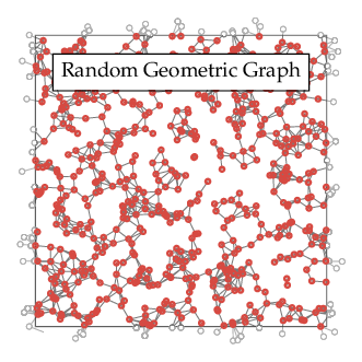
Figure 1. Two-dimensional random geometric graph.
Simulations of disordered systems are particularly demanding from the computational point of view, since on the one hand, large lattice sizes are necessary in order to reduce finite-size corrections and, on the other hand, a large number of independent disorder realizations is required. In the present case, we use linear lattice sizes \(L=8, 10, 12, \ldots, 192\) and simulate \(N_r=10^5\) replicas for the smaller lattices and at least \(N_r=10^4\) for the largest one. Our aim is to use the finite-size scaling of quotients, which allows us to extract the leading correction-to-scaling exponent \(\omega\) to considerable precision. As this method exploits the scaling behavior of observables at the crossing points of phenomenological couplings
$$
R\in{\xi/L, U_{4}, U_{6}, \ldots},
$$
we chose simulation temperatures close to the crossing points of the correlation length in units of the system size, \( \xi/L \). The precise location of the crossing points is then determined via histogram reweighting methods.
As the first step in our analysis, we determine the critical value of the RG invariant quantities as well as the leading correction-to-scaling exponent \(\omega\). This can be done without precise knowledge of the critical temperature and the correlation length exponent \(\nu\), by evaluating the scaling functions at crossing points of \((L,2L)\) pairs of the finite-volume correlation length \(\xi/L\). We use the following scaling ansatz
$$
R|{Q\xi=2}=R^\ast+a_RL^{-\omega},
$$
where sub-leading corrections are neglected, \(R^\ast\) denotes the value of \(R\) at the infinite-volume critical point and the amplitude \(a_R\) of the leading correction term depends on the respective observable used. Uncertainties for the fit parameters are obtained by a comprehensive bootstrap resampling analysis.
| \(L_\text{min}\) | \( (\xi/L)^\ast \) | \( U_4^\ast\) | \(U_6^\ast\) | \(\omega\) | \(\chi^2/\text{d.o.f.}\) |
|---|---|---|---|---|---|
| 8 | 0.5592(11) | 0.6213(2) | 1.4091(16) | 0.451(10) | 3.45 |
| 10 | 0.5618(14) | 0.6208(2) | 1.4134(22) | 0.422(13) | 3.37 |
| 12 | 0.5615(17) | 0.6207(3) | 1.4142(27) | 0.419(16) | 2.42 |
| 16 | 0.5608(28) | 0.6207(5) | 1.4150(43) | 0.419(28) | 1.87 |
| 20 | 0.5596(36) | 0.6208(6) | 1.4141(58) | 0.430(41) | 1.87 |
Table 1. Results of the joint fits mentioned in the text.
When performing individual fits of either \( \xi/L \) or \( U_{4/6} \) according to the above equation, the results turn out to depend quite sensitively on the precise choice of \( L_\text{min} \), specifically \(\omega\) fluctuates in the range 0.3 – 0.5. However, the quality of the fits (and therefore the precision of the \(\omega\) estimate) can be greatly improved by performing a simultaneous fit of all three curves with joint \(\omega\). Results are shown in the upper part of Table 1. Evidently, \(\omega\) only fluctuates very little, as \(L_\text{min}\) is gradually increased. For \(L_\text{min}>16 \), the \(\chi^2/\text{d.o.f.}\) of the fit does not change significantly which indicates that any sub-leading corrections to scaling become small. As our final estimate, we obtain
$$
\omega = 0.42(4),
$$
which includes all individual estimates for \(L_\text{min} = 10,12,16,20\) as well as their corresponding uncertainties. Obviously, this estimate is significantly smaller than the corresponding value for the pure model, \( \omega\approx0.8\) 4, as well as the results found for diluted Heisenberg systems. This already indicates that scaling corrections originating from the topological randomness are considerably strong and necessarily need to be taken into account in the analysis.
Our final estimates for the fixed point values of the phenomenological couplings are hence given by the estimates for \(L_\text{min}=16 \) at the crossing of \( \xi/L \), resulting in
$$
\begin{aligned}
(\xi/L)^* &= 0.5608(28),\
U_4^* &= 0.6207(5),\
U_6^* &= 1.4150(43),
\end{aligned}
$$
which have to be compared to the most-precise values for the Heisenberg model on a cubic lattice, \( (\xi/L)^\ast=0.5644(3) \), \( U_4^\ast=0.6202(1) \) and \( U_6^\ast=1.4202(12) \). All three estimates are compatible, which, already at this stage of the analysis, strongly indicates that our model falls into the same universality class as the pure Heisenberg model. Note, however, that these quantities are only universal in a limit sense as they weakly depend on certain geometrical characteristics of the system.
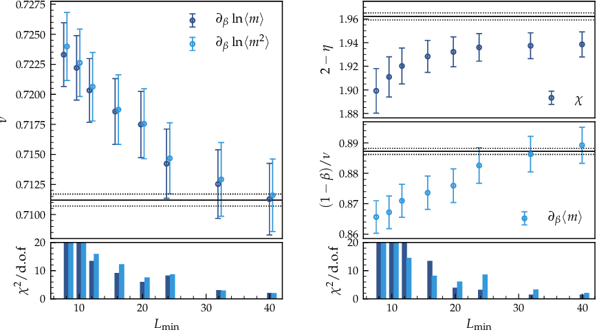
Figure 1. Critical exponents of the three-dimensional Heisenberg model on a RGG. The reduced \\(\chi^2\\) of the fits are indicated in the lower panels on each side. Horizontal lines indicate the reference values and their uncertainties.
Equipped with an estimate for \(\omega\), we are now able to extract critical exponents. This is done by fits to the ansatz
$$
Q_{O}\mid_{ Q_R=s} ,= s^{x_O/\nu} + a L^{-\omega},
$$
where \(x_0/\nu\) denotes the corresponding critical exponent and the quotient is defined by
$$
Q_O = \dfrac{\langle O\rangle (sL,T)}{\langle O\rangle (L,T)}.
$$
In particular, \( \partial\ln\langle m^k\rangle/\partial\beta \), where \( k=1,2 \), yields the correlation length exponent \( \nu \). Furthermore, the susceptibility \( \chi \) allows us to compute \( \gamma/\nu=2-\eta \). Finally, from the magnetization \( \langle m \rangle \) and its derivative \( \partial\langle m\rangle/\partial\beta \), we get the exponents \( \beta/\nu \) and \( (1-\beta)/\nu \), respectively. For all fits we fix \(\omega\) to the estimate computed above, also taking into account its uncertainty. The results are shown in Figure 1. The estimates for \)\nu\) clearly approach the reference value (indicated by the solid horizontal line) for increasing \( L_\text{min} \) and likewise does the exponent \( (1-\beta)/\nu \). In both cases, especially those fits which are – within their uncertainties – compatible with the corresponding reference values, represent the lowest \(\chi^2/\text{d.o.f.}\). The exponent \(\eta\), however, deviates slightly but systematically from its expected value. We hence fit the data for \(\chi\) to the more general ansatz
$$
Q_{\chi}\mid_{ Q_R=s} = s^{\gamma/\nu} + a L^{-\omega}+ b L^{-\omega_2},
$$
introducing an additional higher-order correction term and fixing \(\omega\) as before, hence resulting in four free parameters. From optical inspection of the fits it becomes clear that the largest data point presents itself a considerable outlier, which could be caused the relatively low number of replicas, compared to the magnitude of the disorder. Discarding this point, we find the results listed in Table 2. As can be seen, the estimates are in good agreement with the reference value \(2-\eta=1.9625(5)\). Interestingly, the sub-leading correction exponent is found to be \(\omega_2\approx 2\), although showing considerably large error bars. In fact, this is a reasonable result, since the susceptibility is known to gather corrections proportional to \(L^{2-\eta}\) from its regular background term. Furthermore, since an individual realization of the RGG is not rotationally invariant, corrections proportional to \(\omega_2\approx2\) may also arise from the breaking of the corresponding symmetry.
| \(L_\text{min}\) | \( 2-\eta \) | \( \omega_2\) | \(\chi^2/\text{d.o.f.}\) |
|---|---|---|---|
| 8 | 1.955(8) | 1.68(24) | 4.36 |
| 10 | 1.952(9) | 1.91(47) | 4.23 |
| 12 | 1.953(9) | 1.98(64) | 4.39 |
| 16 | 1.958(13) | 1.95(96) | 4.94 |
| 20 | 1.959(13) | 2.1(11) | 5.95 |
Table 2. Results of the fits of the susceptibility with additional second-order correction term.
In summary, we find a scaling scenario consistent with the clean universal exponents of the Heisenberg universality class, which strongly indicates that the \(O(3)\) symmetric model on a three-dimensional random geometric graph belongs to this class and disorder presents an irrelevant perturbation, as expected. We also find that, owed to the strength of the disorder, corrections to the leading scaling behavior turn out to be considerably strong (\(\omega\approx0.4)\) and necessarily must be taken into account in the analysis.
-
The percolation threshold of the three-dimensional RGG on a torus is located at \(\langle q\rangle = 2.74(1)\), according to Dall, J., & Christensen, M. (2002). Random geometric graphs. Physical review E, 66(1), 016121. ↩︎
-
Campostrini, M., Hasenbusch, M., Pelissetto, A., Rossi, P., & Vicari, E. (2002). Critical exponents and equation of state of the three-dimensional Heisenberg universality class. Physical Review B, 65(14), 144520. ↩︎
-
Gordillo-Guerrero, A., & Ruiz-Lorenzo, J. J. (2007). Self-averaging in the three-dimensional site diluted Heisenberg model at the critical point. Journal of Statistical Mechanics: Theory and Experiment, 2007(06), P06014. ↩︎
-
Guida, R., & Zinn-Justin, J. (1998). Critical exponents of the N-vector model. Journal of Physics A: Mathematical and General, 31(40), 8103. ↩︎