In addition to the Python objects presented in previous sections, pyALF offers a set of scripts that make it easy to leverage pyALF from a Unix shell (e.g. Bash or zsh).
They are located in the folder py_alf/cli, but installation via pip adds entry points to conveniently use them from the Unix shell without further configuration (notably, by trimming the trailing .py).
When starting a code line in Jupyter with an exclamation mark, the line will be interpreted as a shell command.
We will use this feature to demonstrate the shell tools.
2.4.1. alf_run
The script alf_run.py enables most of the features displayed in Section 2.2 to be used directly from the shell. The help text lists all possible arguments:
usage: alf_run [-h] [--alfdir ALFDIR] [--sims_file SIMS_FILE]
               [--branch BRANCH] [--machine MACHINE] [--mpi] [--n_mpi N_MPI]
               [--mpiexec MPIEXEC] [--mpiexec_args MPIEXEC_ARGS]
               [--do_analysis]

Helper script for compiling and running ALF.

options:
  -h, --help            show this help message and exit
  --alfdir ALFDIR       Path to ALF directory. (default: os.getenv('ALF_DIR',
                        './ALF')
  --sims_file SIMS_FILE
                        File defining simulations parameters. Each line starts
                        with the Hamiltonian name and a comma, after wich
                        follows a dict in JSON format for the parameters. A
                        line that says stop can be used to interrupt.
                        (default: './Sims')
  --branch BRANCH       Git branch to checkout.
  --machine MACHINE     Machine configuration (default: 'GNU')
  --mpi                 mpi run
  --n_mpi N_MPI         number of mpi processes (default: 4)
  --mpiexec MPIEXEC     Command used for starting a MPI run (default:
                        'mpiexec')
  --mpiexec_args MPIEXEC_ARGS
                        Additional arguments to MPI executable.
  --do_analysis, --ana  Run default analysis after each simulation.
For example, to run a series of four different simulations of the Kondo model, the first step is to create a file specifying the parameters, with one line per simulation:
Kondo, {"L1": 4, "L2": 4, "Ham_JK": 0.5}
Kondo, {"L1": 4, "L2": 4, "Ham_JK": 1.0}
Kondo, {"L1": 4, "L2": 4, "Ham_JK": 1.5}
Kondo, {"L1": 4, "L2": 4, "Ham_JK": 2.0}
Then, one can execute alf_run.py with options as desired, the script automatically recompiles ALF for each simulation. For understanding some of the options, Section 2.2 might help.
Show code cell output
Hide code cell output
Compiling ALF...
Cleaning up Prog/
Cleaning up Libraries/
Cleaning up Analysis/
Compiling Libraries
ar: creating modules_90.a
ar: creating libqrref.a
Compiling Analysis
Compiling Program
Parsing Hamiltonian parameters
filenames: Hamiltonians/Hamiltonian_Kondo_smod.F90 Hamiltonians/Hamiltonian_Kondo_read_write_parameters.F90
filenames: Hamiltonians/Hamiltonian_Hubbard_smod.F90 Hamiltonians/Hamiltonian_Hubbard_read_write_parameters.F90
filenames: Hamiltonians/Hamiltonian_Hubbard_Plain_Vanilla_smod.F90 Hamiltonians/Hamiltonian_Hubbard_Plain_Vanilla_read_write_parameters.F90
filenames: Hamiltonians/Hamiltonian_tV_smod.F90 Hamiltonians/Hamiltonian_tV_read_write_parameters.F90
filenames: Hamiltonians/Hamiltonian_LRC_smod.F90 Hamiltonians/Hamiltonian_LRC_read_write_parameters.F90
filenames: Hamiltonians/Hamiltonian_Z2_Matter_smod.F90 Hamiltonians/Hamiltonian_Z2_Matter_read_write_parameters.F90
filenames: Hamiltonians/Hamiltonian_Spin_Peierls_smod.F90 Hamiltonians/Hamiltonian_Spin_Peierls_read_write_parameters.F90
Compiling program modules
Done.
Prepare directory "/home/jonas/Programs/pyALF/doc/source/usage/ALF_data/Kondo_L1=4_L2=4_JK=0.5" for Monte Carlo run.
Create new directory.
Run /home/jonas/Programs/ALF/Prog/ALF.out
 ALF Copyright (C) 2016 - 2022 The ALF project contributors
 This Program comes with ABSOLUTELY NO WARRANTY; for details see license.GPL
 This is free software, and you are welcome to redistribute it under certain conditions.
 No initial configuration
Compiling ALF...
Cleaning up Prog/
Cleaning up Libraries/
Cleaning up Analysis/
Compiling Libraries
ar: creating modules_90.a
ar: creating libqrref.a
Compiling Analysis
Compiling Program
Parsing Hamiltonian parameters
filenames: Hamiltonians/Hamiltonian_Kondo_smod.F90 Hamiltonians/Hamiltonian_Kondo_read_write_parameters.F90
filenames: Hamiltonians/Hamiltonian_Hubbard_smod.F90 Hamiltonians/Hamiltonian_Hubbard_read_write_parameters.F90
filenames: Hamiltonians/Hamiltonian_Hubbard_Plain_Vanilla_smod.F90 Hamiltonians/Hamiltonian_Hubbard_Plain_Vanilla_read_write_parameters.F90
filenames: Hamiltonians/Hamiltonian_tV_smod.F90 Hamiltonians/Hamiltonian_tV_read_write_parameters.F90
filenames: Hamiltonians/Hamiltonian_LRC_smod.F90 Hamiltonians/Hamiltonian_LRC_read_write_parameters.F90
filenames: Hamiltonians/Hamiltonian_Z2_Matter_smod.F90 Hamiltonians/Hamiltonian_Z2_Matter_read_write_parameters.F90
filenames: Hamiltonians/Hamiltonian_Spin_Peierls_smod.F90 Hamiltonians/Hamiltonian_Spin_Peierls_read_write_parameters.F90
Compiling program modules
Done.
Prepare directory "/home/jonas/Programs/pyALF/doc/source/usage/ALF_data/Kondo_L1=4_L2=4_JK=1.0" for Monte Carlo run.
Create new directory.
Run /home/jonas/Programs/ALF/Prog/ALF.out
 ALF Copyright (C) 2016 - 2022 The ALF project contributors
 This Program comes with ABSOLUTELY NO WARRANTY; for details see license.GPL
 This is free software, and you are welcome to redistribute it under certain conditions.
 No initial configuration
Compiling ALF...
Cleaning up Prog/
Cleaning up Libraries/
Cleaning up Analysis/
ar: creating modules_90.a
ar: creating libqrref.a
Compiling Analysis
Compiling Program
Parsing Hamiltonian parameters
filenames: Hamiltonians/Hamiltonian_Kondo_smod.F90 Hamiltonians/Hamiltonian_Kondo_read_write_parameters.F90
filenames: Hamiltonians/Hamiltonian_Hubbard_smod.F90 Hamiltonians/Hamiltonian_Hubbard_read_write_parameters.F90
filenames: Hamiltonians/Hamiltonian_Hubbard_Plain_Vanilla_smod.F90 Hamiltonians/Hamiltonian_Hubbard_Plain_Vanilla_read_write_parameters.F90
filenames: Hamiltonians/Hamiltonian_tV_smod.F90 Hamiltonians/Hamiltonian_tV_read_write_parameters.F90
filenames: Hamiltonians/Hamiltonian_LRC_smod.F90 Hamiltonians/Hamiltonian_LRC_read_write_parameters.F90
filenames: Hamiltonians/Hamiltonian_Z2_Matter_smod.F90 Hamiltonians/Hamiltonian_Z2_Matter_read_write_parameters.F90
filenames: Hamiltonians/Hamiltonian_Spin_Peierls_smod.F90 Hamiltonians/Hamiltonian_Spin_Peierls_read_write_parameters.F90
Compiling program modules
Done.
Prepare directory "/home/jonas/Programs/pyALF/doc/source/usage/ALF_data/Kondo_L1=4_L2=4_JK=1.5" for Monte Carlo run.
Create new directory.
Run /home/jonas/Programs/ALF/Prog/ALF.out
 ALF Copyright (C) 2016 - 2022 The ALF project contributors
 This Program comes with ABSOLUTELY NO WARRANTY; for details see license.GPL
 This is free software, and you are welcome to redistribute it under certain conditions.
 No initial configuration
Compiling ALF...
Cleaning up Prog/
Cleaning up Libraries/
Cleaning up Analysis/
ar: creating modules_90.a
ar: creating libqrref.a
Compiling Analysis
Compiling Program
Parsing Hamiltonian parameters
filenames: Hamiltonians/Hamiltonian_Kondo_smod.F90 Hamiltonians/Hamiltonian_Kondo_read_write_parameters.F90
filenames: Hamiltonians/Hamiltonian_Hubbard_smod.F90 Hamiltonians/Hamiltonian_Hubbard_read_write_parameters.F90
filenames: Hamiltonians/Hamiltonian_Hubbard_Plain_Vanilla_smod.F90 Hamiltonians/Hamiltonian_Hubbard_Plain_Vanilla_read_write_parameters.F90
filenames: Hamiltonians/Hamiltonian_tV_smod.F90 Hamiltonians/Hamiltonian_tV_read_write_parameters.F90
filenames: Hamiltonians/Hamiltonian_LRC_smod.F90 Hamiltonians/Hamiltonian_LRC_read_write_parameters.F90
filenames: Hamiltonians/Hamiltonian_Z2_Matter_smod.F90 Hamiltonians/Hamiltonian_Z2_Matter_read_write_parameters.F90
filenames: Hamiltonians/Hamiltonian_Spin_Peierls_smod.F90 Hamiltonians/Hamiltonian_Spin_Peierls_read_write_parameters.F90
Compiling program modules
Done.
Prepare directory "/home/jonas/Programs/pyALF/doc/source/usage/ALF_data/Kondo_L1=4_L2=4_JK=2.0" for Monte Carlo run.
Create new directory.
Run /home/jonas/Programs/ALF/Prog/ALF.out
 ALF Copyright (C) 2016 - 2022 The ALF project contributors
 This Program comes with ABSOLUTELY NO WARRANTY; for details see license.GPL
 This is free software, and you are welcome to redistribute it under certain conditions.
 No initial configuration
2.4.2. alf_postprocess
The script alf_postprocess.py enables most of the features discussed in Section 2.3, except for plotting capabilities, to be used directly from the shell. The help text lists all possible arguments:
usage: alf_postprocess [-h] [--check_warmup] [--check_rebin]
                       [-l CHECK_LIST [CHECK_LIST ...]] [--do_analysis]
                       [--always] [--gather] [--no_tau]
                       [--custom_obs CUSTOM_OBS] [--symmetry SYMMETRY]
                       [directories ...]

Script for postprocessing Monte Carlo bins.

positional arguments:
  directories           Directories to analyze. If empty, analyzes all
                        directories containing file "data.h5" it can find,
                        starting from the current working directory.

options:
  -h, --help            show this help message and exit
  --check_warmup, --warmup
                        Check warmup. Opens new window.
  --check_rebin, --rebin
                        Check rebinning for controlling autocorrelation. Opens
                        new window.
  -l, --check_list CHECK_LIST [CHECK_LIST ...]
                        List of observables to check for warmup and rebinning.
  --do_analysis, --ana  Do analysis.
  --always              Do not skip analysis if parameters and bins are older
                        than results.
  --gather              Gather all analysis results in one file named
                        "gathered.pkl", representing a pickled pandas
                        DataFrame.
  --no_tau              Skip time displaced correlations.
  --custom_obs CUSTOM_OBS
                        File that defines custom observables. This file has to
                        define the object custom_obs, needed by
                        py_alf.analysis. (default: os.getenv("ALF_CUSTOM_OBS",
                        None))
  --symmetry, --sym SYMMETRY
                        File that defines lattice symmetries. This file has to
                        define the object symmetry, needed by py_alf.analysis.
                        (default: None))
To use the symmetrization feature, one needs a file defining the object symmetry, similar to the already used file custom_obs.py defining custom_obs.
"""Define C_4 symmetry (=fourfold rotation) for pyALF analysis."""
from math import pi


# Define list of transformations (Lattice, i) -> new_i
# Default analysis will average over all listed elements
def sym_c4_0(latt, i): return i
def sym_c4_1(latt, i): return latt.rotate(i, pi*0.5)
def sym_c4_2(latt, i): return latt.rotate(i, pi)
def sym_c4_3(latt, i): return latt.rotate(i, pi*1.5)

symmetry = [sym_c4_0, sym_c4_1, sym_c4_2, sym_c4_3]
To analyze the results from the Kondo model and gather them all in one file gathered.pkl, we execute the following command.
Show code cell output
Hide code cell output
### Analyzing ALF_data/Kondo_L1=4_L2=4_JK=0.5 ###
/home/jonas/Programs/pyALF/doc/source/usage
Custom observables:
custom E_squared ['Ener_scal']
custom E_pot_kin ['Pot_scal', 'Kin_scal']
custom SpinZ_pipi ['SpinZ_eq']
Scalar observables:
Constraint_scal
Ener_scal
Kin_scal
Part_scal
Pot_scal
Histogram observables:
Equal time observables:
Den_eq
Dimer_eq
Green_eq
SpinZ_eq
Time displaced observables:
Den_tau
Dimer_tau
Green_tau
Greenf_tau
SpinZ_tau
### Analyzing ALF_data/Kondo_L1=4_L2=4_JK=1.0 ###
/home/jonas/Programs/pyALF/doc/source/usage
Custom observables:
custom E_squared ['Ener_scal']
custom E_pot_kin ['Pot_scal', 'Kin_scal']
custom SpinZ_pipi ['SpinZ_eq']
Scalar observables:
Constraint_scal
Ener_scal
Kin_scal
Part_scal
Pot_scal
Histogram observables:
Equal time observables:
Den_eq
Dimer_eq
Green_eq
SpinZ_eq
Time displaced observables:
Den_tau
Dimer_tau
Green_tau
Greenf_tau
SpinZ_tau
### Analyzing ALF_data/Kondo_L1=4_L2=4_JK=1.5 ###
/home/jonas/Programs/pyALF/doc/source/usage
Custom observables:
custom E_squared ['Ener_scal']
custom E_pot_kin ['Pot_scal', 'Kin_scal']
custom SpinZ_pipi ['SpinZ_eq']
Scalar observables:
Constraint_scal
Ener_scal
Kin_scal
Part_scal
Pot_scal
Histogram observables:
Equal time observables:
Den_eq
Dimer_eq
Green_eq
SpinZ_eq
Time displaced observables:
Den_tau
Dimer_tau
Green_tau
Greenf_tau
SpinZ_tau
### Analyzing ALF_data/Kondo_L1=4_L2=4_JK=2.0 ###
/home/jonas/Programs/pyALF/doc/source/usage
Custom observables:
custom E_squared ['Ener_scal']
custom E_pot_kin ['Pot_scal', 'Kin_scal']
custom SpinZ_pipi ['SpinZ_eq']
Scalar observables:
Constraint_scal
Ener_scal
Kin_scal
Part_scal
Pot_scal
Histogram observables:
Equal time observables:
Den_eq
Dimer_eq
Green_eq
SpinZ_eq
Time displaced observables:
Den_tau
Dimer_tau
Green_tau
Greenf_tau
SpinZ_tau
ALF_data/Kondo_L1=4_L2=4_JK=0.5
No orbital locations saved.
ALF_data/Kondo_L1=4_L2=4_JK=1.0
No orbital locations saved.
ALF_data/Kondo_L1=4_L2=4_JK=1.5
No orbital locations saved.
ALF_data/Kondo_L1=4_L2=4_JK=2.0
No orbital locations saved.
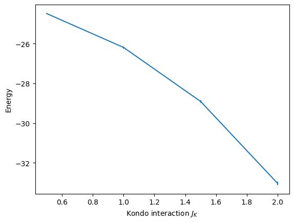
The data from gathered.pkl can, for example, be read and plotted like this: